Building a Basic Quantum Random Walk With Cirq
In this blog post, I’ll be talking a bit about a very interesting application of quantum computing: quantum random walks. Quantum random walks (I’ll shorten this to QRWs throughout the post) are analogous to classical random walks, except the coin function determining the steps that the random walker takes, as well as the position vector of the walker is encoded using qubits and unitary transformations (in other words, we took a regular random walk and translated the main ideas to quantum analogues). If the reader would like to dive deeper into quantum random walks, this is a very good review paper on that key concepts involved in the creation of QRWs: https://arxiv.org/pdf/quant-ph/0303081.pdf.
Classical Random Walks
A random walks is a random process, involving a “walker” that is placed in some -dimensional medium (like a grid or a graph). We then repeatedly query some random variable, and based on the outcome of our measurement, the walker’s position vector (position on the graph or grid) is updated. A very basic example of a random walk is the one-dimensional graphical case, where we consider a marker placed on the origin of a number line with markings at each of the integers. Let the initial position vector of our marker be . For steps of our random walk, so take a set of random variables, , which can take on either a value of or with equal probability (). To find the updated position vector of our walker, we simply compute the value:
Where we know:
So for our case, the final position vector is simply . This model of a random walk can easily be generalized to -dimensions. Another important fact to note is that for a discrete, 1-dimensional random walk on a number-line-like graph, the probability of the random walker being at a specific location follows a binomial distribution. Let us define an -step random walk. Let us then assert that , where is the number of steps to the left, and is the number of steps to the right. We can then reason that if there is some probability of the walker taking a rightward step at one time-step of the random walk, the probability of taking a leftward step is given by . It follows that the probability of taking leftward steps, and rightward steps in a random walk of total steps is given by:
We then have to consider the probability that for an step random walk, our walker ends up at position . Well, we know the probability of taking left steps and right steps, and we know that for a random walk of steps, the position of the walker is determined by the number of left steps, minus the number of right steps. Since it doesn’t matter the order in which the sequence of steps occurs, to find the total probability of being at some location, , we have to multiply the probability by the number of possible ways in which left steps and right steps can be arranged in a sequence. Well, since we have total steps, we can “choose” of those steps to be allocated to rightward steps, and automatically know that the remaining steps were left steps. We calculate “choose” steps by calculating the binomial coefficient, therefore getting:
And so we have shown that the probability distribution for the position of the walker for an step random walk is given by a binomial distribution. This fact is important in the context of this blog post, as we will show that the probability distribution that is created when a quantum random walk is simulated is nowhere close to the binomial distribution that we expect to see for a classical 1-dimensional random walk.
Quantum Random Walks
The process of the quantum random walk isn’t that much different from its classical counterpart, although the observed results of the two processes have many differences. First, let us motivate the creation of a QRW. This part of the theory is completely clear to me as of yet (still something that I’m looking into), but the idea is that when one performs analysis on a classical random walk, you can find that , where is the standard deviation of the random walk’s probability distribution, and is the number of time-steps of the random walk. For the quantum random walk, we can see that . In other words, the standard deviation grows at a quadratically faster rate. At a high level, this signifies that the quantum walker “spreads out” quadratically faster than the classical one, showing that the process of a QRW is quadratically faster than its classical counterpart.
In order to create a quantum random walk, we have to translate the components of the classical random walk to a quantum problem. We can encode the position of a “walker” in some -dimensional space with a vector . For the purpose of this project, we will be investigating a very basic case of a random walk on a ring-shaped graph, with adjacent nodes connected by a single edge. The configuration looks something like this:
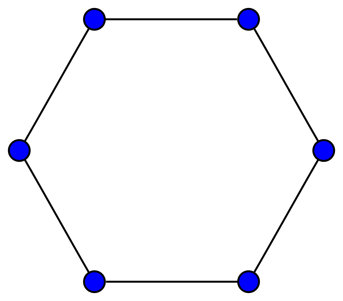
Going back to our original idea of some position vector , it is apparent that in order to encode the location of a “walker” on this graph, we need to assign a specific value of our position vector to each node. Well, this is fairly simple, for a graph of nodes, we form a Hilbert space
spanned by the following set:
We also require another vector in order to create a random walk. We need a “coin vector”, which will encode the direction in which the random walk will progress at the -th step of the process. This Hilbert space is spanned by the two basis states, representing forward and backward progression on our number-line-like graph (actually, I guess our graph looks more like a ring, so I guess our two basis states will represent clockwise and counter-clockwise motion, but it’s the same idea). We will call this Hilbert space , and we can again define our spanning set:
Where the upward-arrow symbol represent counter-clockwise motion, and the downward arrow represents clock-wise motion. Now that we have defined all of the vectors we need to encode the information about our random walk, we must understand how we can realize these vectors in our quantum algorithm. Well, this is again fairly simple. For a graph of nodes, we require qubits to encode binary representations of numbers ranging from to , therefore each of the vectors spanning will simply be given by the binary representation of corresponding to the basis vector . For the coin vector, since we have only two states, we only need one qubit to encode the two possible states:
In order to represent the total space of all possible states of our system, we take the tensor product of the two spanning sets, which will then span the new Hilbert space . We will write a general element of this Hilbert space as
Moving right along, we now require a method to evolve our random walk forward at each step. We define a random walk evolution operator as follows:
By the way, I didn’t come up with this genius operator, this came from the paper I referenced at the top of the post. Essentially, since our qubits take on states and , we know that any possible, general basis state vector formed from qubits will be orthogonal to all other vectors in the basis spanning the space. Because of this, we can create an operator that first “picks out” the coin vector’s state (the other term just goes to , as, like I said, the states or orthogonal), and then sums over all possible position states until it finds the position state to which the operator is being applied. The inner product of the vector and itself is just one (the vectors are not only orthogonal, they’re orthonormal!), and the new position state of the vector is , depending on the state of the coin vector. This did exactly what we wanted, it evolved our random walk either forward or backwards by one step! If you’re still not convinced, let’s check to see what happens when we have the state and we apply the operator:
As you can see, it works! Now, we must consider the randomness of the random walk. For the purposes of our random walk, we will set , and therefore make as well. At each time step, it is necessary that we randomly flip the state of our coin vector . The Hadamard transformation seems like a natural choice, as:
The probability of measuring one of the basis states is given by squaring the coefficient in the linear combination, which we can see for both outcomes is equal to , the same probability of a step to the right/step to the left that we originally desired. We can now combine our operators into one “master operator” that works as one complete step of the random walk, including randomizing the coin vector:
Now that we have defined all of the mathematical machinery with which we are working, we can now begin the implementation of the algorithm! This is where I actually had to start thinking for myself (hahaha), as I had to figure out a way to translate all of the math into an actual quantum circuit. To start, we have to prepare our qubit register. By using qubits, we can create a graph with nodes. We also need an extra qubit for our coin vector, and in addition, we need a register of ancilla qubits (you will see why we need this ancilla later). We can code this up using Cirq:
  qubits = []
  for i in range(0, number_qubits):
      qubits.append(cirq.GridQubit(0, i))

  ancilla = []
  for i in range(0, number_qubits+2):
      ancilla.append(cirq.GridQubit(1, i))


  #The coin vector is defined as cirq.GridQubit(0, number_qubits)
  #and is not contained in either of the lists
Next, we need to decide how we are going to implement the random-walk evolution operator. We can actually do this using a lot of Toffoli, CNOT, and X gates. In order to implement the unitary transformation, we first have to check the value of the coin vector. We can use the fact that our coin vector determines whether a step goes forward or backward in order to implement individual “step forward” and “step backward” gates, both of which are controlled by the coin qubit. First, like we said, before, we apply a Hadamard gate to the coin qubit, then we apply our controlled step forward and step backward gates. Let’s start with the step forward operator. In order to add one step to our position vector, we simply have to add one to the binary representation of our position vector (expressed using the qubits). We start with the least significant qubit. If this qubit is in the state, it will become . If the qubit is in state , the qubit will become and the is carried forward to the next qubit. This process continues for each successive qubit. In order to implement this, we first implement a gate to flip the first qubit conditionally, based on whether the coin qubit is in the up or down state. In order to carry the to the next qubit, if necessary, we implement an gate on the -value qubit, and then a Toffoli gate controlled by the coin qubit, and the $1$-value qubit, controlling the -value. We then apply an gate to the -value qubit, and a 3-qubit controlled CNOT, controlled by the coin qubit, the -value qubit, and the -value qubit, applied to the -value qubit. This pattern continues on for each qubit. After this, we apply a series of gates to every position qubit, in order to reverse the operations that we previously applied. We can define this operation mathematically as:
The notation I’m using here is a bit random, but I’m essentially saying that we are applying we’re applying to the -th position qubit, controlled by all qubit “below” it, along with the coin qubit, then applying an gate to the -th qubit. After this, we apply an gate to each of the position qubits.
In order to implement this process in code, we have to do a couple things. First, we have to define a function for an -qubit Toffoli gate. This is why we introduced the ancilla register at the beginning of the program: it is necessary for this gate:
  def apply_n_qubit_tof(ancilla, args):

      if (len(args) == 2):
          yield cirq.CNOT.on(args[0], args[1])

      elif (len(args) == 3):
          yield cirq.CCX.on(args[0], args[1], args[2])

      else:

          yield cirq.CCX.on(args[0], args[1], ancilla[0])
          for k in range(2, len(args)-1):
              yield cirq.CCX(args[k], ancilla[k-2], ancilla[k-1])

          yield cirq.CNOT.on(ancilla[len(args)-3], args[len(args)-1])

          for k in range(len(args)-2, 1, -1):
              yield cirq.CCX(args[k], ancilla[k-2], ancilla[k-1])
          yield cirq.CCX.on(args[0], args[1], ancilla[0])
We can then prepare our position qubit register to begin halfway between and , where is the number of nodes on the random-walk graph:
  def initial_state():

      yield cirq.X.on(cirq.GridQubit(0, 1))
We then have to apply the step forward operator:
  def walk_step():

      #Start by applying the coin operator to the flip qubit

      #Implement the Addition Operator

      yield cirq.H.on(cirq.GridQubit(0, number_qubits))

      for i in range(number_qubits, 0, -1):

          yield apply_n_qubit_tof(ancilla, [cirq.GridQubit(0, v) for v in range(number_qubits, i-2, -1)])
          yield cirq.X.on(cirq.GridQubit(0, i-1))

      for i in range(number_qubits+1, 1, -1):
          yield cirq.X.on(cirq.GridQubit(0, i-1))
But this is only half the story, we also need a “step backwards” step operator. Well, luckily, quantum computational operators are reversible, meaning that in order to implement a subtraction operator, all we have to do is literally apply our addition operator, but in reverse order!! Since these operators are controlled by the coin qubit, we apply an gate to the coin qubit, and then use it as a control qubit for the second operator (the step backwards operator):
  def walk_step():

      #Start by applying the coin operator to the flip qubit

      #Implement the Addition Operator

      yield cirq.H.on(cirq.GridQubit(0, number_qubits))

      for i in range(number_qubits, 0, -1):

          yield apply_n_qubit_tof(ancilla, [cirq.GridQubit(0, v) for v in range(number_qubits, i-2, -1)])
          yield cirq.X.on(cirq.GridQubit(0, i-1))

      for i in range(number_qubits+1, 1, -1):
          yield cirq.X.on(cirq.GridQubit(0, i-1))

      #Implement the Substraction Operator

      yield cirq.X.on(cirq.GridQubit(0, number_qubits))

      for i in range(number_qubits+1, 1, -1):
          yield cirq.X.on(cirq.GridQubit(0, i-1))

      for i in range(1, number_qubits+1):

          yield apply_n_qubit_tof(ancilla, [cirq.GridQubit(0, v) for v in range(number_qubits, i-2, -1)])
          yield cirq.X.on(cirq.GridQubit(0, i-1))
We then build our circuit, and simulate it!
  circuit = cirq.Circuit()

  circuit.append(initial_state())

  for j in range(0, number_of_steps):
      circuit.append(walk_step())
  circuit.append(cirq.measure(*qubits, key='x'))

  simulator = cirq.Simulator()
  result = simulator.run(circuit, repetitions=number_of_repetitions)
  final = result.histogram(key='x')
Finally, let’s graph the probability distribution of the position of our random walker by using matplotlib:
  x_arr = [j for j in dict(final).keys()]
  y_arr = [dict(final)[j] for j in dict(final).keys()]

  x_arr_final = []
  y_arr_final = []

  while (len(x_arr) > 0):

      x_arr_final.append(min(x_arr))
      y_arr_final.append(y_arr[x_arr.index(min(x_arr))])
      holder = x_arr.index(min(x_arr))
      del x_arr[holder]
      del y_arr[holder]

  plt.plot(x_arr_final, y_arr_final)
  plt.scatter(x_arr_final, y_arr_final)
  plt.show()
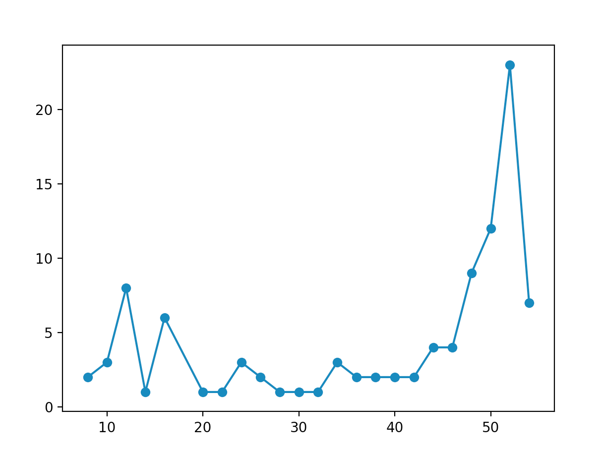
Now, let’s take a look at the result! As it turns out, the overall shape of the probability distribution is a lot different than the binomial distribution that we derived earlier! In fact, the probability distribution depends on the initial state of the coin qubit! For the initial state of (where we have a graph of nodes), we generate a probability distribution that looks like this (after 30 steps of the program, for 100 trials):
And for the initial state of , we get:
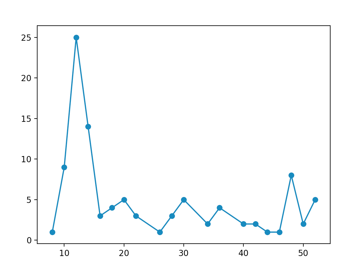
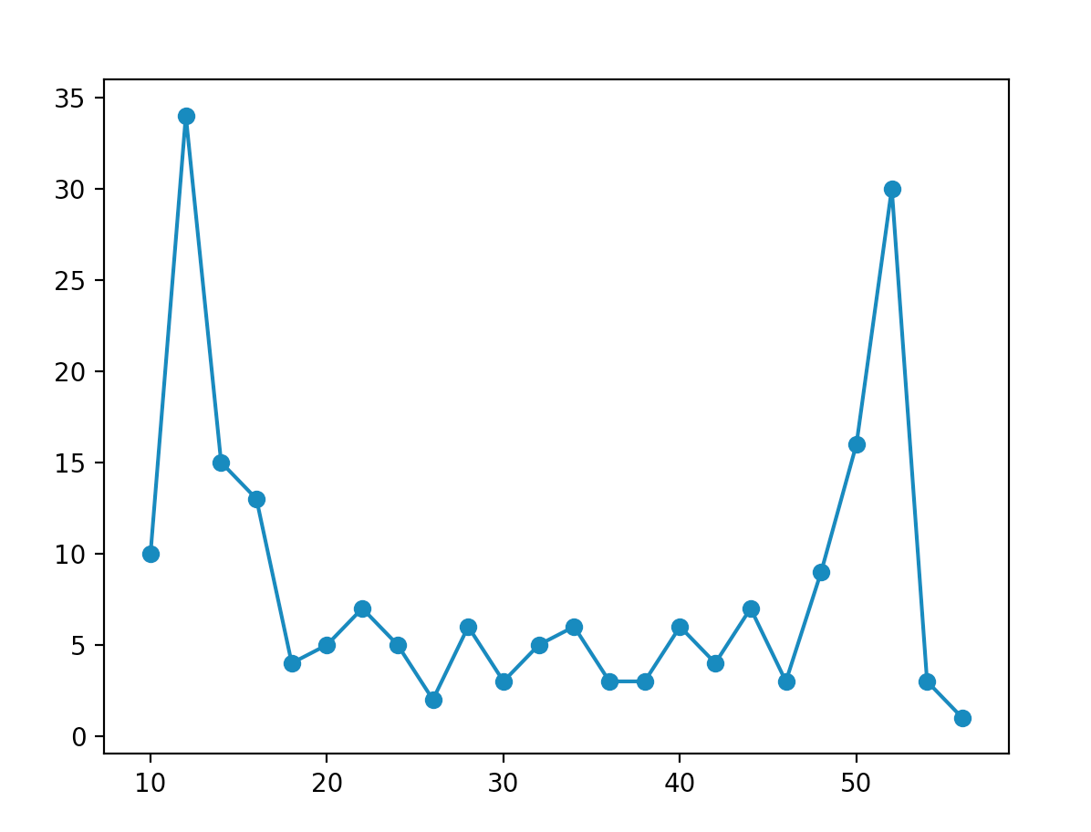
As you can see, these distributions show a large spike near one end, and a smaller spike at the other (in other words, nothing like a binomial distribution)!! The reason why we get this distribution is because when we continue to apply Hadamard gates to a qubit without measuring it after each application, the probability amplitudes of the different states interfere constructively and destructively with each other in interesting ways. I’m not going to do this math in this post, but if you don’t believe me, pick an initial state and apply four or five Hadamard transformations to it, then check the probabilities of measuring different states. We can actually choose an initial state that gives us a ssymetric probability distribution, which looks something like this:
This is because the imaginary and real parts of the state vector don’t interfere in the same fashion, and thus we get a probability distribution that looks like this (I had to increase the number of trials to 200 to get a nice-looking probability distribution):
To just wrap up this article, I just want to say that I have barely scratched the surface of quantum random walks. It is a fascinating application of quantum computation that I am just beginning to look into. Ultimately, random walks have tons of applications in the real world, in areas ranging from biology to finance. Due to the computational speedup, QRWs could actually be very impactful once quantum hardware becomes more robust to errors and allows us to scale to more qubits, and for this reason, I’m going to ocntinue to dive deeper into QRWs! Stay tuned for further content!
If you are interested, here is the link to the Github repo with the full code for the QRW! https://github.com/Lucaman99/Cirq-Quantum-Computing/blob/master/qrw/qrw.py