Continuous QAOA Optimization with Photonic Quantum Computation: A Tutorial

Disclaimer: I am not entirely sure whether my implementation of this algorithm is correct. I basically read this research paper and attempted the translate the math into an actual quantum circuit. If this post is suddenly deleted, it means that I have found a mistake in my work, and I have to revise this post (fear not, if this happens, I will definitely re-post with the correct information). Anyways, let’s get to the fun stuff.

Continuous variable optimization is an area of great interest, especially in the context of quantum computation. The reason for this is that right now, we are aware of the fact that quantum computation optimization algorithms are able to demonstrate a computational speedup over their classical counterparts. However, most of the implementations of these optimization algorithms have been done using discrete quantum computation (quantum computation with qubits). This is a good method for optimization, and can approximate the optimization of continuous functions to a certain extent, but ion order to effectively optimize continuous functions, and continuous-variable optimization algorithm must be used.

In order to create a continuous-variable implementation of QAOA, we can use a photonic quantum computational algorithm. In this tutorial, I will implement the algorithm using the Strawberry Fields library for photonic quantum computing. Each optical mode in the simulation will correspond to one parameter which is being optimized. For the purpose of our implementation, we are only optimizing one parameter, $x$ , therefore we only need to use one mode.

This purpose of this post is to act as a tutorial on implementing the continuous-variable QAOA algorithm outlined in the previously mentioned paper. For the purpose of this tutorial, I am going to be implementing the algorithm for a basic function, just a parabola that has been shifted by some factor which we will call $a$ :

$$f(x) \ = \ (x \ - \ a)^2$$

To begin our algorithm, we have to initialize our mode (which represents the parameter we are optimizing). The guys who wrote this paper are very smart. They initialized the modes to a squeezed state, which will increase the variance of the $\hat{x}$ quadrature, therefore having a greater likelihood of overlapping with our desired solution (I should clarify, to measure the resulting output of this algorithm, we perform a X-Homodyne measurement of the mode). For my simulation, a decided to set the squeezing parameter of this state to $r \ = \ -0.5$ , which squeezes the mode along its $\hat{p}$ quadrature and stretches it in $\hat{x}$ . Coding this up in Strawberry Fields, we have:

    with eng:
        Squeezed(-0.5,0) | q[0]

Now, we move into the bulk of the algorithm. In order to implement QAOA, we need to choose two Hamiltonians, a cost ( $H_C$ ) and a non-commuting mixer ( $H_M$ ) (this is in line with the mechanism of the originally proposed discrete-variable QAOA, as outlined in this paper). These Hamiltonians are then applied repeatedly to the initial state, one after the other, for a fixed number of steps which we call $P$ . This means that we define our evolutionary evolution for one step of the program to be:

$$U(\alpha, \ \beta)_{i} \ = \ e^{-i\alpha_i H_{M}} \ e^{-i\beta_i H_{C}}$$

The reason for this is that the general form of a unitary transformation is $U \ = \ e^{-iK}$ . Since we know our Hamiltonians are Hermitian, we get valid unitaries to apply in our quantum circuit. Where the total evolution of the wavefunction in our quantum circuit is of the form:

$$|\psi\rangle \ \rightarrow \ |\psi'\rangle \ = \ \Big( \displaystyle\prod_{s \ = \ 1}^{P} \ U(\alpha, \ \beta)_{s}\Big) \ |\psi\rangle$$

Where $\alpha$ and $\beta$ are sets (indexed by $i$ ) of constant parameters that dictate the evolution of our system (these parameters actually correspond to more concrete, recognizable phenomenon, like the learning rate in the gradient descent algorithm, but I’m not going to talk about that here. To learn more, take a look at the paper referenced at the beginning of this post).

Since the cost Hamiltonian corresponds to a function that we are trying to optimize, we can write it in the form of the function we are attempting to optimize, but in terms of the $\hat{x}$ -quadrature, as this is the parameter we are optimizing and measuring. This means that we have:

$$H_M \ = \ f(\hat{x}) \ = \ (\hat{x} \ - \ a)^2 \ = \ \hat{x}^2 \ - \ 2a\hat{x} \ + \ a^2$$

And our corresponding unitary:

$$U_C \ = \ e^{-i\beta_i (\hat{x}^2 \ - \ 2a\hat{x} \ + \ a^2)} \ = \ e^{-i\beta_i \hat{x}^2} e^{i\beta_i 2a\hat{x}} e^{-i\beta_i a^2} \ = \ e^{-i\beta_i \hat{x}^2} e^{i\beta_i 2a\hat{x}}$$

Notice how I eliminated the constant multiplier $e^{-i\beta_i a^2}$ , as it is just an overall phase and has no effect on the state. Now, let us consider the mixer Hamiltonian. We will use one of the examples provided in the paper, the number Hamiltonian, which is of the form:

$$H_M \ = \ \displaystyle\sum_{i \ = \ 1}^{N} \ \hat{a}^{\dagger}_i \hat{a}_i$$

Where $N$ is the number of modes in our circuit, and $\hat{a}$ and $\hat{a}^{\dagger}$ are the creation and annihilation operators. Since we are only working with one mode, we have:

$$U_M \ = \ e^{-i \alpha_i \hat{a}^{\dagger}_i \hat{a}_i}$$

We have to consider now how we will implement these unitaries in a quantum circuit. Well this is actually simpler than it seems, we need to find optical quantum gates that correspond to three different unitaries: $e^{-i\beta_i \hat{x}^2}, \ e^{i\beta_i 2a\hat{x}}, \ \text{and} \ e^{-i \alpha_i \hat{a}^{\dagger}_i \hat{a}_i}$ . Well luckily, these unitaries are of the same form as three common optical quantum gates: the quadratic phase gate, the momentum displacement gate, and the rotation gate, defined respectively as follows:

$$P(s) \ = \ e^{i\frac{s}{2\hbar}\hat{x}^2}$$ $$Z(p) \ = \ e^{ip\hat{x}/\hbar}$$ $$R(\phi) \ = \ e^{i\phi\hat{a}^{\dagger}_i \hat{a}_i}$$

Doing some simple algebra and setting $\hbar \ = \ 2$ , we get:

$$s_i \ = \ -4 \beta_i$$ $$p_i \ = \ 4a\beta_i$$ $$\phi_i \ = \ -\alpha_i$$

We can then implement this in Strawberry Fields code, building off of the code for our initial state. For this implementation, we will make a function that we can repeatedly call based on the value of $P$ :

def run_circuit(alpha_param, beta_param, parabolic_min):

    with eng:

        Squeezed(-0.5,0) | q[0]

        Zgate(parabolic_min*4*beta_param[0]) | q[0]
        Pgate(-4*beta_param[0]) | q[0]
        Rgate(-1*alpha_param[0]) | q[0]
        Zgate(parabolic_min*4*beta_param[1]) | q[0]
        Pgate(-4*beta_param[1]) | q[0]
        Rgate(-1*alpha_param[1]) | q[0]
        Zgate(parabolic_min*4*beta_param[2]) | q[0]
        Pgate(-4*beta_param[2]) | q[0]
        Rgate(-1*alpha_param[2]) | q[0]

        MeasureX | q[0]

        state = eng.run('gaussian', cutoff_dim=5)

    return q[0].val

Where alpha_param and beta_param are our sets of parameters, and parabolic_min is our value of $a$ . After this, all that is left to do is measure our mode with an $X$ -Homodyne measurement.

Now, in order to find optimal values for our sets of parameters $\alpha$ and $\beta$ , I have taken a fairly simple approach and simply sample from a pre-defined list of constant values for a fixed number of iterations. After the program chooses a set of parameters (randomly), it runs the program a fixed number of times, taking an average of these trials, and then calculating the “loss” of the obtained value. If this loss is less than the loss for previous iterations, the value of the “optimal parameters” is updated, along with the variable we are trying to optimize, $x$ . When this part of the program completes, the optimal $\alpha$ and $\beta$ sets are taken, and are repeatedly run, and an average is taken, to make sure that the chosen $\alpha$ and $\beta$ yield a probability distribution that is close to the expected optimized value of our function (this part of the algorithm is more for testing purposes). Here is the complete code for my simulation, including the method that I used to find optimal values of $\alpha$ and $\beta$ :

import strawberryfields as sf
from strawberryfields.ops import *
from strawberryfields.utils import scale
from numpy import pi, sqrt
import math
import random

from matplotlib import pyplot as plt

eng, q = sf.Engine(1)


iterations = 45
shots = 10
parabolic_min = 3
possible_parameters = [0.1, 0.3, 0.5, 0.7, 0.9, 1.1]
testing_trials = 100
optimal_value = math.inf
simulation = []

#Calculating loss

def function_optimize(x, parabolic_min):
    y = (x - parabolic_min)**2
    return y

#Run the photonic quantum circuit

def run_circuit(alpha_param, beta_param, parabolic_min):

    with eng:

        Squeezed(-0.5,0) | q[0]

        Zgate(parabolic_min*4*beta_param[0]) | q[0]
        Pgate(-4*beta_param[0]) | q[0]
        Rgate(-1*alpha_param[0]) | q[0]
        Zgate(parabolic_min*4*beta_param[1]) | q[0]
        Pgate(-4*beta_param[1]) | q[0]
        Rgate(-1*alpha_param[1]) | q[0]
        Zgate(parabolic_min*4*beta_param[2]) | q[0]
        Pgate(-4*beta_param[2]) | q[0]
        Rgate(-1*alpha_param[2]) | q[0]

        MeasureX | q[0]

        state = eng.run('gaussian', cutoff_dim=5)

    return q[0].val

#Search for the optimal value

op = 0

alpha_param = [0.5, 0.5, 0.5]
beta_param = [0.5, 0.5, 0.5]

for i in range(0, iterations):
    result = 0
    grid = []
    for h in range(0, shots):
        hello = run_circuit(alpha_param, beta_param, parabolic_min)
        result = result+hello
        grid.append(hello)
    result = result/shots
    calculation = function_optimize(result, parabolic_min)

    yer_a = alpha_param
    yer_b = beta_param

    if (calculation < optimal_value):
        simulation = grid
        optimal_value = calculation
        the_x_measurement = result
        op = [[alpha_param[0], alpha_param[1], alpha_param[2]], [beta_param[0], beta_param[1], beta_param[2]]]

    alpha_param[0] = possible_parameters[random.randint(0, len(possible_parameters)-1)]
    alpha_param[1] = possible_parameters[random.randint(0, len(possible_parameters)-1)]
    alpha_param[2] = possible_parameters[random.randint(0, len(possible_parameters)-1)]

    beta_param[0] = possible_parameters[random.randint(0, len(possible_parameters)-1)]
    beta_param[1] = possible_parameters[random.randint(0, len(possible_parameters)-1)]
    beta_param[2] = possible_parameters[random.randint(0, len(possible_parameters)-1)]


optimal_parameters = op


x_arr = range(0, testing_trials)
y_arr = []

for i in range(0, testing_trials):

    state = run_circuit(optimal_parameters[0], optimal_parameters[1], parabolic_min)
    y_arr.append(state)

print(y_arr)

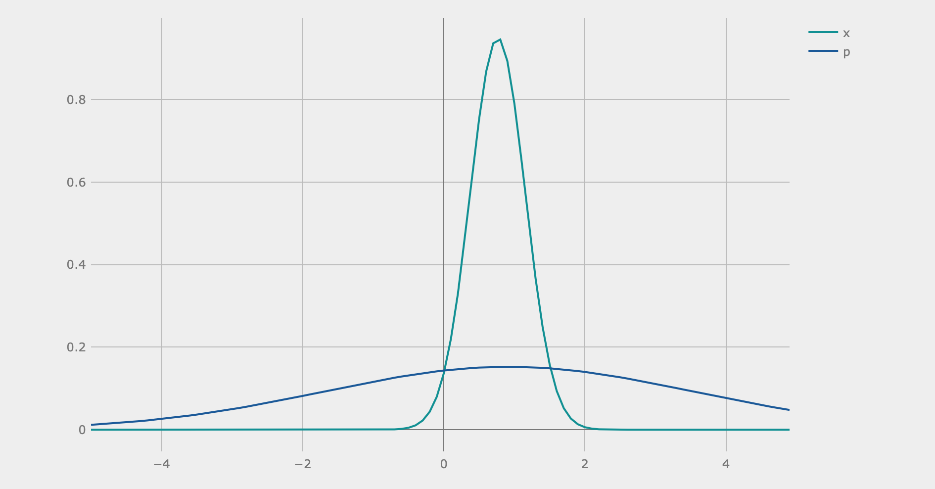
The algorithm seems to work pretty well. Here is an example of the quadrature plots when I ran the algorithm with $a \ = \ 1$ . I was able to generate these graphs by inputting optimized parameters yielded from my program to the Strawberry Fields interactive simulation interface (the blue-green graph is the $\hat{x}$ -quadrature):

First Step of the Algorithm

first

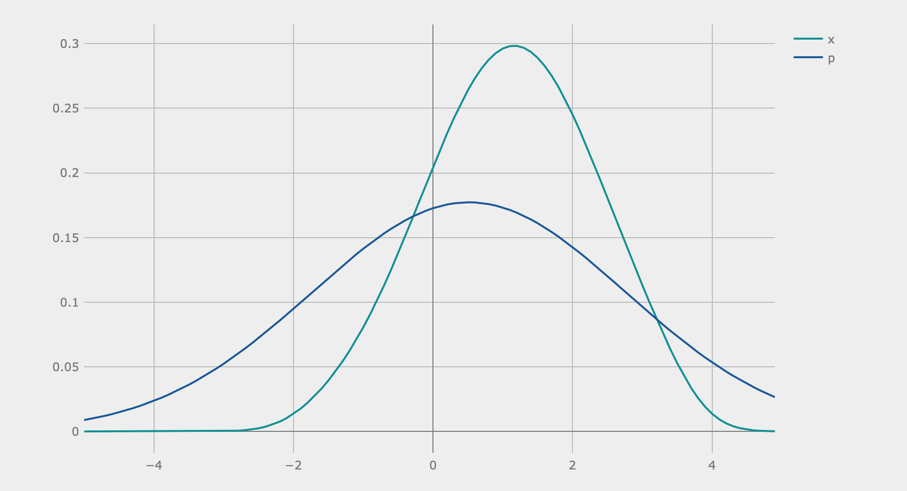
Second Step of the Algorithm

first

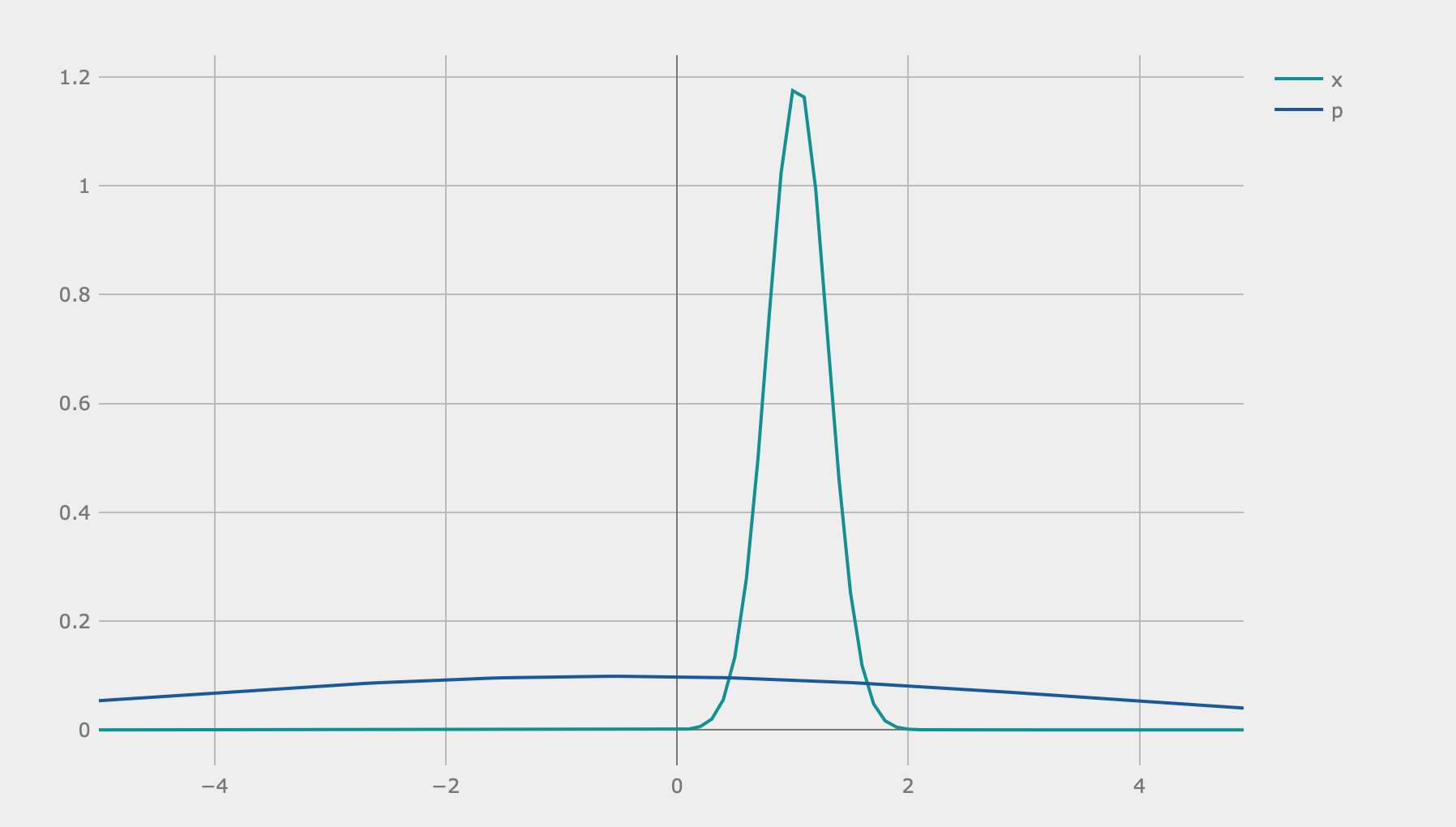
Third Step of the Algorithm

first

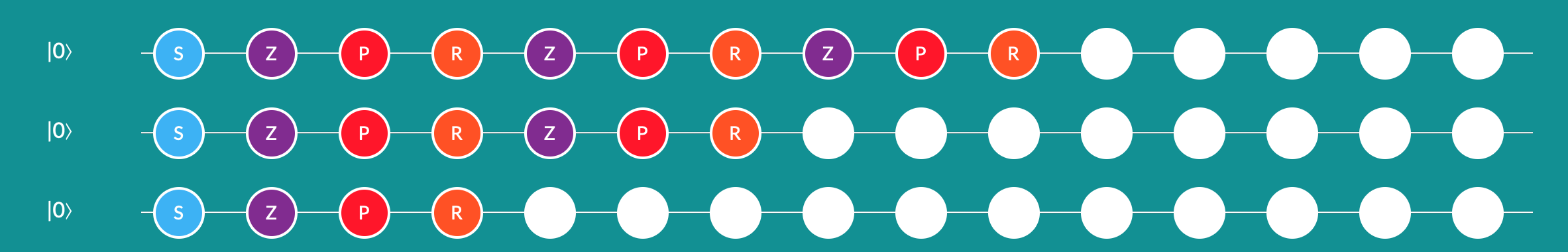
The Circuits I Used to Generate These Three Graphs

first

As can be seen, after three steps, the peak of the $\hat{x}$ -quadrature is located at around $\hat{x} \ = \ 1$ , which is the expected optimal value of our function. Keep in mind that the algorithm does not work a lot of the time, as not all values of $\alpha$ and $\beta$ actually lead to circuits that correctly find the optimal value. These values have to be chosen based on the context of the problem being solved/function being optimized.

Thank you for reading my post! If you liked this content, check out my personal website for more projects and articles!