Inferno Tutorial: Cumulative Tree Burn Graph
In this post, I will be briefly describing a tutorial for generating some interesting data using the first release of Inferno v0.0.1(b). What we will be looking at today is a number which I am calling the cumulative burn total. This is just some function C(t), that maps to the total number of trees that have burned on a forest grid up until time t. For this tutorial, we will be examining this function only in the case of a random grid.
We can start by specifying some function which will generate our graph of C(t) versus t. We will write this function in the form cumulative_burn_sum(length, width, tree_density, iterations), where the first three keywords are simply entered into the random forest generation function as parameters, and the iterations parameter represents how many times we want our function to simulate a forest (as we will get more accurate results if we average together the simulation repeated multiple times).
We can then write our repeated simulation of the forest as:
def cumulative_burn_sum(length, width, tree_density, iterations):
    max_length = 0
    final = []
    for n in range(0, iterations):
        g = inferno.CreateRandomGrid(length, width, tree_density, 0, 0)
        fire = inferno.spread_random_fire(g)
The reason for the two variables defined outside of our for-loop will become apparent later in the tutorial. If we are going to plot on the x-axis, time, it is important for us to know how many time-steps our simulation took, so we will add the following code within our for-loop, to find this maximum value of t by searching through our burnt forest:
maximum = 0
    for i in fire:
        if (i[3] > maximum):
            maximum = i[3]
In addition to finding this maximum value of t, we also want to find how many trees have burned at each time step, so we add this code within our for loop (as we want to repeat this process for each forest that is generated) that cycles through our burnt grid, checking to see at what time-step each of the trees burnt at, adding it to a counter variable, and then appending this counter variable to a list after checking one value of t. In addition, we are also interested in finding the maximum length of all of our simulations (the one with the most time-steps), because in order to average together all of our simulations, we need all of them to have the same dimension, so we have to append some extra numbers to the end of some of our lists, to ensure they are all the same length:
y = []
    add = 0
    for i in range(0, maximum+1):
        for j in fire:
            if (j[3] == i and j[2] == 1):
                add = add + 1
        y.append(add)
    if (len(y) > max_length):
        max_length = len(y)
    final.append(y)

tell = final
Next, we are going to add extra final[i][len(final[i])-1] entries to the end of each of the datasets final[i] that have a length less than the maximum. We are doing this because in the time-steps after the fire has burnt out, the fire isn’t spreading anywhere new, so the number of squares burnt after this burnout time will remain constant into the future. Recall that we already know our max length, so this task is fairly easy (this block of code is outside the original for-loop, as we are done cycling through each of our data-sets; we have all the data we need to for each of the individual simulations):
append_arr = []

for i in range (0, len(final)):
    counting = 0
    for n in range(0, max_length-len(final[i])):
        final[i].append(final[i][len(final[i])-1])
        counting = counting+1
    append_arr.append(counting)
Next, we average together all the lists containg the number of trees burned at each time-step:
all = [sum(v) for v in zip(*list(final))]
all_two = [a/iterations for a in all]
Where all_two is our final, averaged list. Finally, we can plot the results using matplotlib:
x = range(0, len(all_two))
plt.plot(x, all_two)
plt.show()
And we’re done! Let’s try it out. For the example of cumulative_burn_sum(50, 50, 2500, 10) we get something that looks like this:
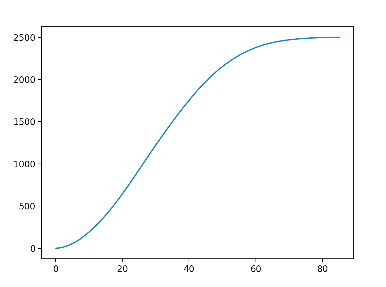
This is super cool! You can use this code to play around more with different tree densities, forest sizes, and even modify it slightly to simulate even and clustered forests. All together, the final code for this tutorial looks like this:
import inferno
from matplotlib import pyplot as plt
import math

def cumulative_burn_sum(length, width, tree_density, iterations):
    max_length = 0
    final = []
    for n in range(0, iterations):
        g = inferno.CreateRandomGrid(length, width, tree_density, 0, 0)
        fire = inferno.spread_random_fire(g)
        maximum = 0
        for i in fire:
            if (i[3] > maximum):
                maximum = i[3]

        y = []
        add = 0
        for i in range(0, maximum+1):
            for j in fire:
                if (j[3] == i and j[2] == 1):
                    add = add + 1
            y.append(add)
        if (len(y) > max_length):
            max_length = len(y)
        final.append(y)

    tell = final

    append_arr = []

    for i in range (0, len(final)):
        counting = 0
        for n in range(0, max_length-len(final[i])):
            final[i].append(final[i][len(final[i])-1])
            counting = counting+1
        append_arr.append(counting)

    all = [sum(v) for v in zip(*list(final))]
    all_two = [a/iterations for a in all]

    x = range(0, len(all_two))
    plt.plot(x, the_chosen_one)
    plt.show()

cumulative_burn_sum(50, 50, 2500, 10)
Thank you for reading! If you liked this tutorial and have an questions or feedback, please do not hesitate to reach out to me at jackceroni@gmail.com. I will be putting out more content like this as we continue to roll out new features in Inferno!