March 16, 2020

In this blog post, we are going to turn our attention to interesting combinatorial graph theory problems, and how they can be solved with QAOA. This blog post won't go through what QAOA is and why it works. Rather, we will focus more on graph theory, and the interesting problems that arise when we consider different colourings/characteristics of the graph, while also creating some toy simulations of QAOA being used to solve some of these problems. Disclaimer: I am not claiming that the mathematical methods I used to construct the cost functions corresponding to these problems in the most efficient: I simply wanted to use this blog post as a place to write down everything I havee learned while trying to independently arrive at a decently-good method for solving these problems (except for MaxCut, that method had already been beat into my mind from previous reading)

---

Preliminary Stuff: NetworkX and My Graph Code

We can start this post by simpling writing a little bit of code that will allow us to construct graphs a bit more easily while running our simulations. We will make use of the Python library, NetworkX, along with some custom classes that we will write up ourselves. We can start by defining classes that allows us to construct graph and graph-edge objects. We can then define a simple graph and save it as an image for Matplotlib and NetworkX:

For the specific example of the edges that we inputted into the program, we get a graph that looks something like this:

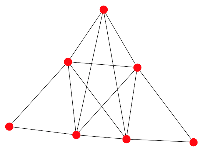
A cool looking graph

We will make good use of this small piece of code throughout this blog post.

QAOA MaxCut

The first use case of QAOA that we are going to look into is the MaxCut problem. This problem is as follows: given some undirected graph $G \ = \ (V, \ E)$, find the cut that passes through $S \ \subset \ E$, such that $|S|$ is maximized. A cut is defined as a partition of the nodes of a graph into two subsets, $A$ and $B$, such that $A \ \cup \ B \ = \ V$ and $A \ \cap \ B \ = \ \emptyset$. To determine $|S|$, we can look at each $a \ \in \ A$. If there exists some $b \ \in \ B$ such that $(a, \ b) \ \in \ E$, then we add $1$ to $|S|$, continuing this process until we have checked all $a$.

An equivalent way to formulate this problem is through the language of graph colouring. Consider, instead of thinking about partitioning in terms of a cut, we create partitions based on whether we colour specific nodes of our graph black or white. Thus, we have two sets of nodes, $W$ for white and $B$ for black, such that $W \ \cup \ B \ = \ V$ and $W \ \cap \ B \ = \ \emptyset$. We wish to maximize the number of edges that end in nodes that have different colourings. We can construct this by considering each $w \ \in \ W$. If there exists some $b \ \in \ B$, such that $(w, \ b) \ \in \ E$, then we know that we have an edge with different-coloured endings, and we add $1$ to our "score". Looking back, this is completely equivalent to the "cutting" formulation of this problem.

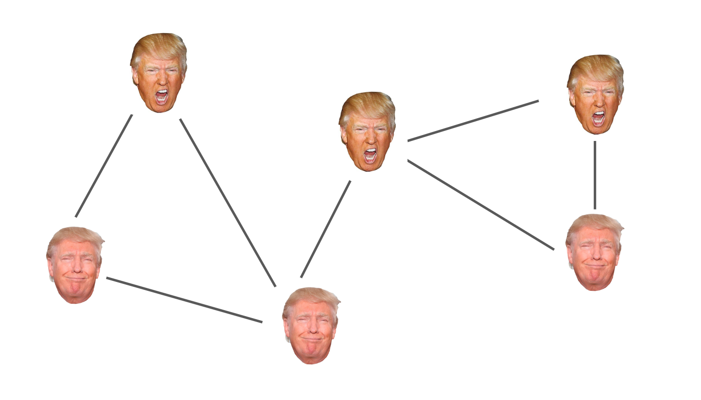
A whimsical MaxCut graph colouring

As it turns out, the problem of figuring out this partition of nodes is a computationally difficult problem (NP-complete). Despite this, the near-term quantum algorithm, QAOA, is pretty good at solving these types of problems. QAOA actually doesn't show any speedup for small graphs like the ones we will investigate in this post, but nevertheless, it is a fun idea to think about.

Since this post assumes you are already familiar with QAOA, I will jump right into choosing cost and mixer Hamiltonian for our alternating unitary layers. We will turn our attention to the cost Hamiltonian first. Recall that we are interested in finding the colouring of our graph that yields the maximum number of edges with endings of different colours. Thus, it would make sense for our cost function to "reward" edges with different-coloured endings, and do nothing when the endings are the same colour. In fact, we can quantify this. Let's say that $-1$ is added to our overall cost function when adjacent nodes have different colours, and $0$ when they are the same (as we are trying to minimize our cost function).

We also know that within a quantum computer, our qubits, when measured, take on one of the computational basis states corresponding to the basis in which we are performing measurement. For each individual qubit, that "basis value" can be denoted by $0$ or $1$. Thus, for each individual qubit $|0\rangle$ corresponds to a black colouring, and $|1\rangle$ corresponds to a white colouring. However, in , we are not going to use $0$ and $1$, instead using $1$ and $-1$, respectively, in their place (the reasoning for this will become apparent very soon). Thus, we assign $1$ to a black colouring of a node and $-1$ to a white colouring of a node. We then define our cost function as follows:

$$C \ = \ \displaystyle\sum_{a, \ b} \ \frac{1}{2} (c_a c_b \ - \ 1) \ \ \ \ \ (a, \ b) \ \in \ E$$
Where $c_a$ and $c_b$ represent colourings of vertex $a$ and vertex $b$ respectively. As you can check for yourself, when $c_a \ \neq \ c_b$, we get a value of $-1$, and when $c_a \ = \ c_b$, we get $0$. Our cost function then sums over all $a$ and $b$ that are joined by an edge.

Now that we have a "classical" cost function, we can map it to the language of quantum computing. This essentially means that we need to map the $c_n$ "function" that tells us the colouring of a specific node to some operator. This is sort of like an analogue of a function: an operator takes its eigenvectors as "argument" and assigns each of them an eigenvalue. We can then calculate the expectation value of that operator with respect to our state to get a "weighted average" of all the different values of the function that could have been measured, with respect to our state.

Luckily, the $Z$ operator is exactly the tool we need to accomplish this. In case you forgot, $Z \ = \ \text{diag}(1, \ -1)$, so it is easy to see that the eigenvalues are $1$ and $-1$, with eigenvectors $|0\rangle$ and $|1\rangle$ respectively. Thus, in order to create a cost Hamiltonian that acts upon states representing vertices coloured black and white, all we have to do is sub out, the $c_a$ and $c_b$ variables for $Z_a$ and $Z_b$. Thus, we get:

$$\hat{H}_C \ = \ \displaystyle\sum_{a, \ b} \ \frac{1}{2} (Z_a \ \otimes \ Z_b \ - \ \mathbb{I}) \ \ \ \ \ (a, \ b) \ \in \ E$$
We can easily verify that this operator acting on pairs of basis states, $|00\rangle$, $|01\rangle$, $|10\rangle$, and $|11\rangle$ yields the expected values of $-1$ and $0$.

In order to choose our mixer Hamiltonian, the general strategy is to find something that does not commute with $\hat{H}_C$, so that the algorithm is able to explore all possibilities in the search space. Consider what would happen in $\hat{H}_{M}$ did commute with $\hat{H}_C$, and each value of our spectrum is unique to a specific eigenvector (which they are). This would imply, $|\psi\rangle$ is an eigenstate of $\hat{H}_C$ if and only if it is an eigenstate of $\hat{H}_M$. Let $|\psi\rangle$ be an eigenstate of $\hat{H}_C$:

$$\hat{H}_M \hat{H}_C \ - \ \hat{H}_C \hat{H}_M \ = \ 0 \ \Rightarrow \ \hat{H}_M \hat{H}_C |\psi\rangle \ - \ \hat{H}_C \hat{H}_M |\psi\rangle \ = \ 0 \ \Rightarrow \ \hat{H}_C [ \hat{H}_M |\psi\rangle ] \ = \ C [ \hat{H}_M |\psi\rangle ]$$
So $\hat{H}_M |\psi\rangle$ is also an eigenvector of $\hat{H}_C$. Let the set $V$ correspond to all eigenvectors of $\hat{H}_C$. It follows that $\hat{H}_M |\psi\rangle \ \in \ aV$, where $a$ is some scaling value. This is to say that $\hat{H}_M$ maps our current eigenvector $|\psi\rangle$ to some new eigenvector, $|\psi'\rangle$, or $\hat{H}_M$ simply scales $|\psi\rangle$ by some factor $a$. However, since we know that each value of the spectrum is unique to a single eigenvector, we c an rule out $\hat{H}_M |\psi\rangle \ = \ |\psi'\rangle$, as if this were true then we would have:

$$\hat{H}_C \hat{H}_M |\psi\rangle \ = \ \hat{H}_M \hat{H}_C |\psi\rangle \ \Rightarrow \ \hat{H}_{C} |\psi'\rangle \ = \ C |\psi'\rangle$$
This is a contradiction, as $C$ is already the eigenvalue assigned to $|\psi\rangle$. Thus, it follows that $\hat{H}_M |\psi\rangle \ = \ a |\psi\rangle$, making $|\psi\rangle$ an eigenvector of $\hat{H}_M$. We can prove the converse in an essentially identical way.

Since the two Hamiltonians share the same set of eigenvectors, this means that there is no "exploration" when a state vector is passed into the circuit. Consider what happens when we pass some general $|\psi\rangle$ into our circuit. This can be decomposed into a linear combination of eigenvectors of the two Hamiltonians. Thus, each term in the linear combination simply has phases multiplied by each term. This is due to the fact that our unitaries are of the form $e^{-i \omega \hat{H}}$, which becomes $e^{-i \omega E}$ when multiplied by one of the eigenstates of $\hat{H}$. Since only adding these phases does not affect the overall probabilities of measurements for any given state, our algorithm is useless (we might as well just randomlly guess solutions).

That was a slight diversion, let's get back on track now. We choose our mixer:

$$\hat{H}_M \ = \ \displaystyle\sum_{n} X_{n}$$
Where $n$ sums over all qubits. Evidently, this does not commute with $\hat{H}_C$.

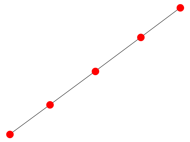
So now that we have defined all of the necessary structure to build our algorithm, let's simulate it using Cirq! First, let's choose the graph on which we are going to perform MaxCut. For the sake of simplicity, we choose a linear graph of $5$ nodes that looks something like this:

We can start by importing all of the necessary libraries, specifying all of the initial parameters that we need, and defining a function that gives us our initial state, which will just be an even superposition of all basis states (high variance in the initial state is good for "exploration", plus, we can motivate that from an adiabatic perspective, as this state is the ground state of $\hat{H}_M$). We'll start with QAOA over $5$ qubits, with a depth of $4$:

We can then go on to define our cost and mixer layers, exactly as we explained them in the previous section:

After this, we can create a function that executes our circuit over multiple trials, and outputs lists of the bitstrings that were measured:

Now, we are able to create our cost function, in order to post-process the data measured from the quantum circuit executions. Since the values that are outputted from the circuit are $0$s and $1$s, instead of the desired $1$ and $-1$ values. Thus, in the place of $c_n$, we defined a function $f(x) \ = \ 1 \ - \ 2x$, which maps $0$ to $1$ and $1$ to $-1$:

This function outputs the expected value of the cost function (calculate the average cost over $1000$ repetitions of the algorithm). Finally, we can define a classical optimizer to tune the $\gamma$ and $\alpha$ paramters until we arrive at a minimum expected value of the cost function. Along with the cost function, we write a bit of code that allows us to graph the results:

When we run the algorithm, the graph of probabilities corresponding to each possible bitstring looks something like this:

Evidently, the states with highest probability of measurement are $|10\rangle \ = \ |01010\rangle$ and $|21\rangle \ = \ |10101\rangle$. These are the two optimal solutions to MaxCut: the vertices are coloured in an alternating fashion, therefore making it such that every edge ends in nodes of different colours (the existence of this "perfect" solution definitely not always possible, for more complex graph).

If we want, we can also turn up the number of nodes in our graph, and get some even cooler looking probability-plots:

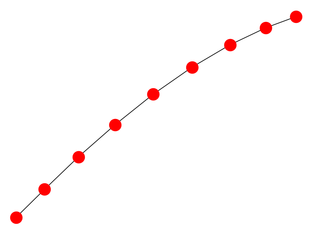
The $n \ = \ 9$ linear graph

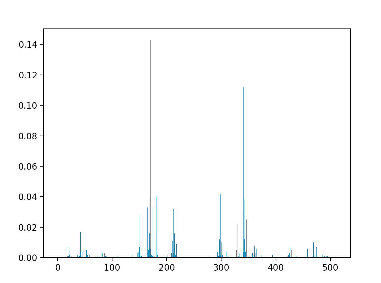
MaxCut on a linear graph for $n \ = \ 9$

As can been seen in the image, there are two large spikes at $|170\rangle \ = \ |010101010\rangle$ and $|341\rangle \ = \ |101010101\rangle$, exactly the results that we expect. We can also look at more interesting graphs, like the one shown at the beginning of the blog post:

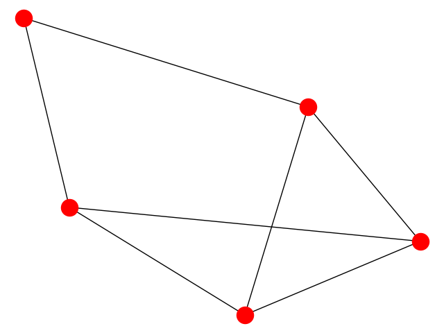
Another cool graph

MaxCut on the cool graph

The results give us $|10\rangle \ = \ |01010\rangle$ and $|21\rangle \ = \ |10101\rangle$ (interestingly enough, the same results as the previous graph). Both of these have MaxCut values of $-6$, which is in fact the maximum possible cut (if you're not convinced, study the graph for a bit and try to find a larger cut. Imagine how difficult this would be for graphs $10$x larger!).

QAOA MaxClique

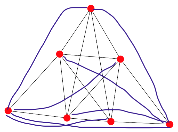
Moving right along, let's look at a slightly more interesting problem, along with some more complex graphs. This time, we are going to look at a problem called MaxClique. Essentially, the the goal of MaxClique is to identify the laargest clique within some arbitrary grahph, $G \ = \ (V, \ E)$. A clique is defined as a subgraph $S \ \subset \ G$, such that for every $v, \ w \ \in \ V(S)$, there exists some $e \ \in \ E(S)$, such that $(v, \ w) \ = \ e$. This is called complete connectedness of our subgraph: every possible pair of nodes is connected by an edge. To shed some light on what this actually looks like, consider the graph that we constructed at the beginning of this post:

The cool graph returns!

As you might be able to see, the largest clique within this graph is surrounded by the pentagon, in the middle. Each node in this subgraph is connected to every other node in the subgraph.

This problem may seem much harder than QAOA MaxCut, but with a bit of mathematical maneuvering, it actually is pretty intuitive! Let's first consider "what" we have to minimize in order to get the maximum clique. Well, first of all, we want the maximum clique, meaning that we want the largest clique possible. Thus, it would make sense for our Hamiltonian to have a part that attempts to penalize small chosen subgraphs and reward large ones. In addition, we also need to make sure that our chosen subgraph is actually a clique. Thus, we write our Hamiltonian as the sum:

$$\hat{H}_C \ = \ \hat{H}_{\text{Max}} \ + \ \omega \ \hat{H}_{\text{Clique}}$$
Where $\omega$ is some real number (the purpose of this number will be explained later). We will label vertices that are contained within our subgraph with $1$, and vertices that are not in our subgraph with $0$. It will be a fairly simple task to find $\hat{H}_{\text{Max}}$: all we need to do is reward instances where we have more $1$s in our bitstring! Thus, we have:

$$\hat{H}_{\text{Max}} \ = \ \displaystyle\sum_{n} Z_{n}$$
Where $n$ sums over all qubits. This means that $-1$ added to the value of our cost when one qubit has a value of $|1\rangle$, and $1$ when a qubit has a value of $|0\rangle$. One can then see that the cost function will be lower when the number of $1$s in the resulting bitstring is greater.

So defining $\hat{H}_{\text{Max}}$ wasn't too difficult, however, we're not done quite yet. We still have to figure our how to define $\text{H}_{\text{Clique}}$, which is suppoed to penalize our resulting bitstring if the subgrapn of $1$s doesn't represent a clique. Consider the graph on which we are performing MaxClique, $G$. Recall the definition of a clique: a subgraph with complete connectedness. This means that every node within the subgraph is connected to every other node within the subgraph. Since we are labelling nodes contained within the subgraph with $|1\rangle$, the definition of a clique asserts that every qubit in the $|1\rangle$ state should be connected to every other qubit in the $|1\rangle$ state. This means that we should penalize every instance of two qubits being in the state $|1\rangle$, that are not connected by an edge of $G$. We take $\bar{G}$ to be the complaiment of $G$, where:

$$\bar{G} \ = \ (V, \ E(K^{|V|}) \ - \ E) \ \ \ \ \ G \ = \ (V, \ E)$$
Where $K^n$ is the complete graph with $n$ vertices. In plain English, $\bar{G}$ is the graph of all edges that are contained within the complete graph determined by $V$ (every node connected to every other node), but not contained within $E$. For example, look at the graph that we showed above. The complaiment of this graph looks like the purple lines here:

$\bar{G}$ is the graph that we will eventually have to sum over when constructing $\hat{H}_{\text{Clique}}$, but before we do that, we first need to find a function that penalizes the pair $|11\rangle$, and rewards or does nothing to pairs $|00\rangle, \ |01\rangle, \ |10\rangle$. This is pretty much equivalent to constructing a boolean $AND$ gate. Like before, in order to take advantage of the eigenvalues of the $Z$ operator, we are going to input values $1$ and $-1$ into our cost function, corresponding to $|0\rangle$ and $|1\rangle$ respectively.

Technically, one could construct this cost function by constructing a discrete polynomial of order $6$, with roots are $|00\rangle$, $|01\rangle$, and $|10\rangle$, but that seems unecessarily painful. We know that our cost function will probably not be too "high-order", and we also know that terms of $x^2$ will make no difference as $-1$ squared and $1$ squared are the same. Thus, we make a half-educated guess that our cost function for a pair of node will be of the form:

$$C(x, \ y) \ = \ a xy \ + \ bx \ + \ cy \ + \ d$$
We then vary the coefficients until we get the desired outputs. In this case, we find that:

$$C(x, \ y) \ = \ \frac{xy \ - \ x \ - \ y \ - \ 1}{2}$$
For inputs of $(1, \ 1)$, $(-1, \ 1)$, and $(-1, \ 1)$ we get a value of $-1$, while for the pair $(-1, \ -1)$, we get a value of $1$. We can eliminate $-1/2$, as it ends up just becoming and overall phase, not affecting our final answer. We are now in the position to define $\hat{H}_{\text{Clique}}$:

$$\hat{H}_{\text{Clique}} \ = \ \displaystyle\sum_{a, \ b} \frac{Z_a \ \otimes \ Z_b \ - \ Z_a \ - \ Z_b}{2} \ \ \ \ \ \ a, \ b \ \in \ V(\bar{G})$$
So all together, we have:

$$\hat{H}_{C} \ = \ \displaystyle\sum_{n} Z_{n} \ + \ \omega \ \displaystyle\sum_{a, \ b} \frac{Z_a \ \otimes \ Z_b \ - \ Z_a \ - \ Z_b}{2}$$
The reason we have $\omega$ is because the "clique part" of the Hamiltonian is more important than the "max part". We could have all the ones in the world, but if our subgraph isn't even a clique to begin with, we have to reject this solution. We call the clique-ness of our solution a hard constraint and the max-ness of our solution a soft constraint. We want to weight the hard constraint higher in our Hamiltonian, so we scale it up by some factor. If we choose $\omega$ to be $2$, we get rid of the denominator in $\hat{H}_{\text{Clique}}$, and we make the bad solution "cost" a lot more, thus we have $\omega \ = \ 2$, and:

$$\hat{H}_{C} \ = \ \displaystyle\sum_{n} Z_{n} \ + \ \displaystyle\sum_{a, \ b} Z_a \ \otimes \ Z_b \ - \ Z_a \ - \ Z_b$$
Again, we choose our mixer Hamiltonian to simply to a sum of $X$ operations over all qubits in the circuit. We can now begin writing up our simulations! We won't rewrite all of the previous code for qubit initialization and the mixer unitary, so we begin by writing a small method that identifies $\bar{G}$:

We then go on to define the new cost unitary:

Finally, we go on to define the new cost function. Recall that thee output from the circuit is in terms of $0$ and $1$ rather than $1$ and $-1$, so we use our previously defined function $f(x)$ to map to the correct set of numbers:

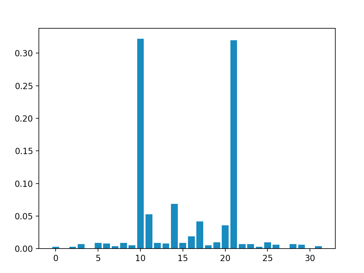
Using this code, combined with the code from the previous MaxCut section, we can run MaxClique on a bunch of different graphs. First, let's try finding the maximum clique of the "cool graph" that we have been using through this section. Running this simulation, we get a graph that looks something like this:

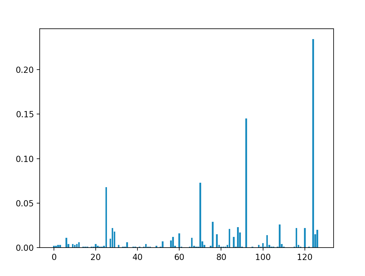
As you can see, the tallest spike corresponds to $|124\rangle \ = \ |1111100\rangle$, which is exactly the answer we expect (the way we labelled the qubits make qubits $1$, $2$, $3$, $4$, and $5$ the middle pentagon). It is possible to perform MaxClique for more complicated graphs, with increased circuit depth, but for now, we are going to leave those simulations to the reader and move on to the next QAOA application.

QAOA Travelling Salesman Problem

The travelling salesman problem is defined as follows : given a graph $G \ = \ (V, \ E)$, along with a metric $D_{E}(e)$ that assigns distances to each $e \ \in \ E$, what is the path, $P$, that includes all $v \ \in \ V$, such that:

$$C \ = \ \displaystyle\sum \ D_{E}(p) \ \ \ \forall p \ \in \ P$$

is minimized? A path is defined as some ordered list of edges, such that each edge is only included once in the list. This problem is the most daunting one that we will tackle with QAOA in this blog post. In order to solve this, we first need to come up with a good encoding scheme for the problem. The optimally chosen path, along with the list $V$ is going to be a subgraph of $G$, with each vertex connected to $2$ other vertices, to form a ring-shaped structure. We are going to use this constraint during our construction of the cost function, but firstly, let us define our encoding scheme to be bitstrings representing an adjacency matrix corresponding to our subgraph. For a graph $G$, with $n \ = \ |V(G)|$, the adjacency matrix, $A$, will be an $n \ \times \ n$ matrix, such that some matrix element $A_{ij}$ is set to $1$ if there exists an edge between vertex $i$ and vertex $j$, and $0$ is there exists no such edge. For example, for the "cool graph" in the previous section, the adjacency matrix is defined as:

$$A \ = \ \begin{pmatrix} 0 & 1 & 1 & 1 & 1 & 1 & 0 \\ 1 & 0 & 1 & 1 & 1 & 0 & 1 \\ 1 & 1 & 0 & 1 & 1 & 0 & 1 \\ 1 & 1 & 1 & 0 & 1 & 1 & 0 \\ 1 & 1 & 1 & 1 & 0 & 0 & 0 \\ 1 & 0 & 0 & 0 & 1 & 0 & 0 \\ 0 & 0 & 1 & 1 & 0 & 0 & 0 \end{pmatrix}$$

So when we define our path, it would make sense to also use an adjacency matrix, where the number of $1$s in a given row is equal to $2$. Now, we must consider the cost function itself. We wish to minimize the distance travelled along the given path, thus we should just used the originally defined $C$ as our cost function. Each value associated with $D_E$ can be stored in some look-up table that we reference when constructing our circuit. Thus, we define this part of our cost Hamiltonian as:

$$\hat{H} \ = \ \displaystyle\sum_{i, \ j} \ \frac{D_{ij}}{2} (1 \ - \ Z_{ij})$$

Where $D_{ij}$ is the distance of the edge between vertex $i$ and vertex $j$, and $Z_{ij}$ is the $Z$ gate on the qubit corresponding to the $i$-th row and $j$-th column of the adjacency matrix. However, this cost function says nothing about the hard constraint, which is that each row of the adjacency matrix must have only two entries equal to $1$. We will thus borrow a technique used in this paper: "A quantum alternating operator ansatz with hard and soft constraints for lattice protein folding". Essentially, we want to encode the hard contraints of our problem in the mixer unitary, such that only the state-space of feasible solutions is explored. In this case, it will be the states where the Hamming weight (sum of binary digits) of each row of the adjacency matrix is equal to $2$. In order to actually do this, we will initialize our qubit register in an even superposition of qubit state with Hamming weight two (I'll talk more about this soon), and we define our mixer to be the generalized SWAP gate, used in the referenced paper. This gate preserves Hamming weight, and is defined as:

$$SWAP_{i, \ j} \ = \ \frac{1}{2} (X_i X_j \ + \ Y_i Y_j)$$

So we define our mixer Hamiltonian as:

$$\hat{H}_M \ = \ \displaystyle\sum_{i, \ j} \ SWAP_{i, \ j} \ = \ \displaystyle\sum_{i, \ j} \ \frac{1}{2} (X_i X_j \ + \ Y_i Y_j)$$

Where we apply the terms between adjacent qubits. Now, going back to our initial desire to initialize our qubits in an even superposition of all bitstrings of Hamming weight $2$, I am not smart enough to think of any rhyme or reason to the method that I have found to initialize these bitstrings, but essentially it just comes down to intuitively thinking of the $\sqrt{SWAP}$ gate as something that has a $50\%$ chance of swapping qubits (while adding some local phases in the process), and trying to "balance" out the probabilities of all bitstrings of a given Hamming weight, then correcting for the local phases with exponential $Z$ gates. The initialization circuits that we will use for TSP aren't exact (the probabilities of measuring the feasable bitstrings are different), however, with this initialization we restrict ourselves to the subspace of feasable bitstrings. The subsequent layers of unitaries will hopefully correct for the non-uniform initialized probabilities, as we pass the initial state through the QAOA circuit. 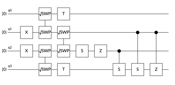There is definitely an initialization circuit such that the initial probabilities for each of feasable bitstrings are equal, so if you are reading this and bothered by the "slopiness" of this step, by all means try to find the "more-correct" circuit. For now, we are going to attempt to do TSP with $3$ nodes, thus the initialization circuit that we use for each "row" of the adjacnecy matrix will look something like:

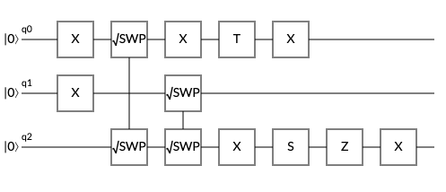
For this initialization circuit, we correct for the different phases with the single quibts applied after the $\sqrt{SWAP}$ gates, however, the initial probability distribution is not uniform.

In order to proceed, there is also one other hard constraint that we must consider: the fact that our bitstrings have to represent an actual adjacency matrix. Allow me to elaborate, consider the following matrix:

$$A \ = \ \begin{pmatrix} 0 & 0 & 0 & 0 & 0 & 1 & 1 \\ 0 & 0 & 0 & 0 & 0 & 1 & 1 \\ 0 & 0 & 0 & 0 & 0 & 1 & 1 \\ 0 & 0 & 0 & 0 & 0 & 1 & 1 \\ 0 & 0 & 0 & 0 & 0 & 1 & 1 \\ 0 & 0 & 0 & 0 & 0 & 1 & 1 \\ 0 & 0 & 0 & 0 & 0 & 1 & 1 \end{pmatrix}$$

This is definitely not an adjacency matrix. For instance, the top right entry of the matrix says that vertex $1$ is connected to vertex $7$, however, there is not a $1$ in the bottom left corner, which signifies the same information and should be present. Thus, the idea behind our new penalty, which essentially checks if the outputted bitstring is a valid adjacency matrix is that we apply $ZZ$ operations between qubits that represent reflection of one-another across the main diagonal of the adjacency matrix. In other words:

$$\hat{H}' \ = \ - \displaystyle\sum_{a, \ b} Z_a Z_b \ \ \ \ \ a \ = \ A_{ij} \ \ \ b \ = \ A_{ji}$$

And we thus arrive at our final cost Hamiltonian:

$$\hat{H}_C \ = \ \hat{H} \ + \ \hat{H}' \ = \ \displaystyle\sum_{i, \ j} \ \frac{D_{ij}}{2} (1 \ - \ Z_{ij}) \ - \ \omega \displaystyle\sum_{a, \ b} Z_a Z_b$$

Summing over all elements $A_{ij}$, except for those on the main diagonal of the adjacency matrix. We can drop away the overall phase that is being added to each qubit (even though the phase is different, they all sum together to give the same effect on each of the basis states). Thus, we are simply left with:

$$\hat{H}_{C} \ = \ - \frac{1}{2} \displaystyle\sum_{i, \ j} \ D_{ij} Z_{ij} \ - \ \omega \displaystyle\sum_{a, \ b} Z_a Z_b$$

Let's choose $\omega$ to be relatively large. Like before, we want to ensure that the hard-constraints are always satisfied. Thus, let's choose $\omega \ = \ 5$, and define our cost unitary:

$$\hat{U}_C \ = \ e^{i\gamma \big(\frac{1}{2} \sum_{i, \ j} \ D_{ij} Z_{ij} \ + \ 5 \sum_{a, \ b} Z_a Z_b \big)} \ = \ e^{i \gamma \frac{1}{2} \sum_{i, \ j} \ D_{ij} Z_{ij}} e^{5 i \gamma \sum_{a, \ b} Z_a Z_b} \ = \ \displaystyle\prod_{i, \ j} e^{i \frac{\gamma}{2} D_{ij} Z_{ij}} \ \displaystyle\prod_{a, \ b} e^{5 i \gamma Z_{a} Z_{b}}$$

We can also define our new mixer unitary:

$$\hat{U}_M \ = \ e^{-i \frac{\alpha}{2} \sum_{i, \ j} (X_i X_j \ + \ Y_i Y_j)} \ = \ \displaystyle\prod_{i, \ j} e^{-i \frac{\alpha}{2} X_i X_j} e^{-i \frac{\alpha}{2} Y_i Y_j}$$

With all of this, we can now begin creating our simulations of QAOA TSP. For now, we are going to investigate a practically trivial problem, with only $3$ vertices. This will require $9$ qubits (which is a lot, and really puts in persepctive the quadratic scaling of qubits that I'm using in this implementation). Anyways, continuing on, we can first write up some code that gives us the initialization circuit:

We can then define the new cost unitary subroutine. In order to do this, we use "distance" and "coupling" lists, which we define for a specific graph later:

We also define our new mixer unitary:

And finally, we define our new cost function:

And without further delay, we can test out our TSP algorithm on a simple graph. We'll first investigate the trivial case of a $3$-node graph.

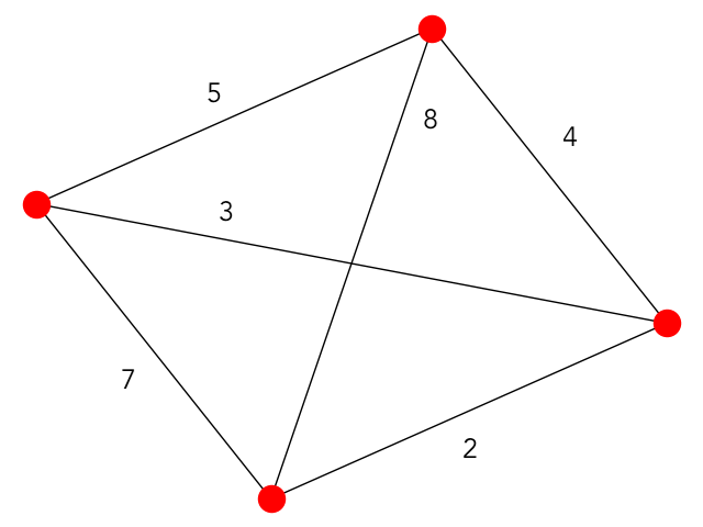
We'll consider the following weighted graph:

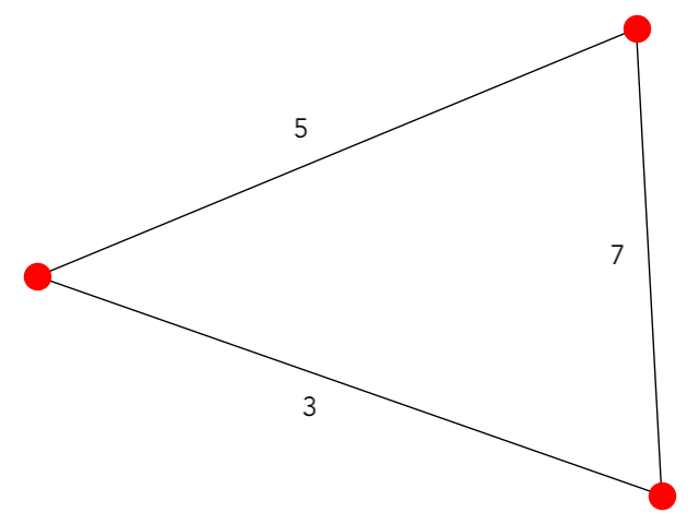
This problem is beyond trivial, there is literally only one choice for a path through this graph, but nevertheless, we will perform TSP on it. First, let us define the distance matrix for this graph:

$$D \ = \ \begin{pmatrix} 15 & 5 & 3 \\ 5 & 15 & 4 \\ 3 & 4 & 15 \end{pmatrix}$$

We chose the digagnal elemnts to be large, as we want to "repel" our simulation away from placing $1$s on the diagonal of adjacency matrix (as we previously explained). The "coupling" list included within our code just includes a list of all pairs that are reflections of each other across the main diagonal of a $3 \ \times \ 3$ matrix. Now, just as a test we can take graph a plot of our cost function for all feasable bitstrings (bitstrings that don't represent possible adjacency matrices aren't included in this plot):

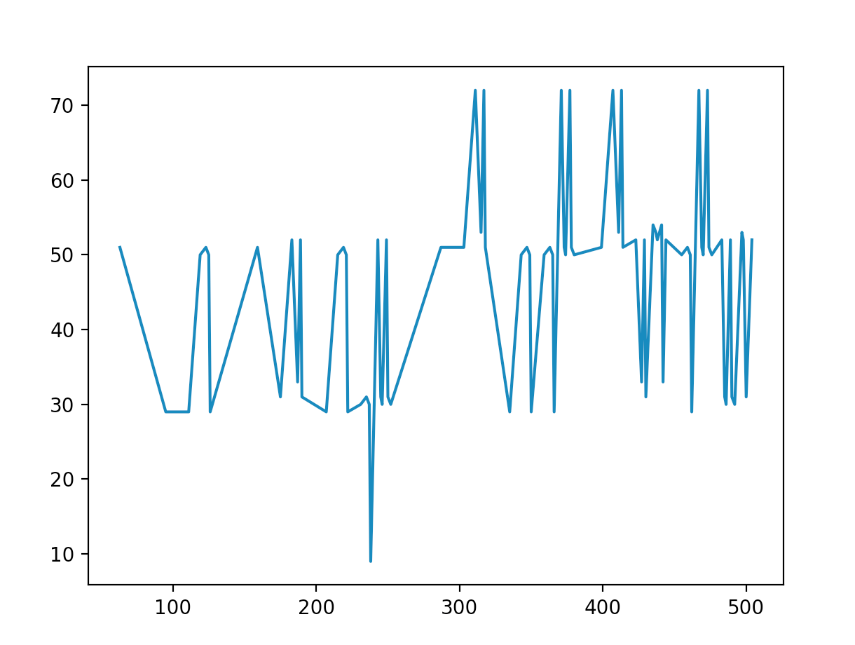
As you can see, our cost function takes on its minimum value at $x \ = \ 238$, which we will soon see is in fact the correct solution to the TSP problem we have outlined. Finally, we can encode this information and the graph easily into our pre-existing "graph code", and run the simulation, getting a probability distribution that looks something like this:

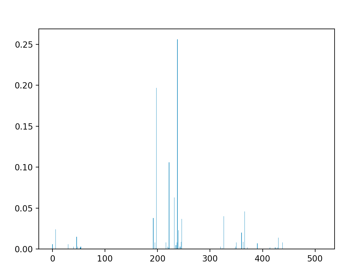
As can be seen, the tallest spike (the highest probability) lies at the state $|238\rangle \ = \ |011101110\rangle$. We can translate this into a matrix:

$$A \ = \ \begin{pmatrix} 0 & 1 & 1 \\ 1 & 0 & 1 \\ 1 & 1 & 0 \end{pmatrix}$$

Which is exactly the path that through the matrix, thus $|238\rangle$ is the correct solution. It is important to note that for this simulation, instead of setting the search space to $(-\pi, \ \pi)$, we instead used $\Big( -\frac{\pi}{4}, \ \frac{\pi}{4} \Big)$ (motivated by the fact that for this simulation, our circuit depth was $4$). This was the only way to get the simulations to converge well (previous tests of this algorithm for the larger search space were incredibly volatile, in terms of the resulting distribution). This may be explained by the fact that the initial state is far from optimal, the search space of the mixers is already constrained to an extent such that altering amplitudes requires finer adjustments to converge, or that TSP is an inherently volatile problem that requires increased circuit depth and/or better tuning of parameters in the cost function. All of these possible faults could be remedied, and I believe that the algorithm would perform even better if we made these corrections (in this blog post, we will not spend time doing that, but the eager reader of this post may be interested in trying to increase the quality of the simulations).

To conclude all of our TSP simulations, let's attempt to solve a problem that is slightly less trivial than the one that we just did: a $4$ vertex graph. Specifically, we will investigate:

We will use pretty much the exact same code as before, with the same restrictions on the search space, and a new distance matrix that encodes all of the edges of this particular graph. The only thing that changes is the initialization circuit, which now needs to accomodate $4$ qubits:

Again, this circuit does not yield an even distribution over all feasable states, and is probably not optimized, but it serves its function: restricting us to the subspace of realizable solutions. We won't display the cost function for this instance of TSP, because frankly, the range is too large to render and actually zoom in on the minima (I tried). Instead, we will jump directly to running QAOA TSP. We get a distribution that looks something like this:

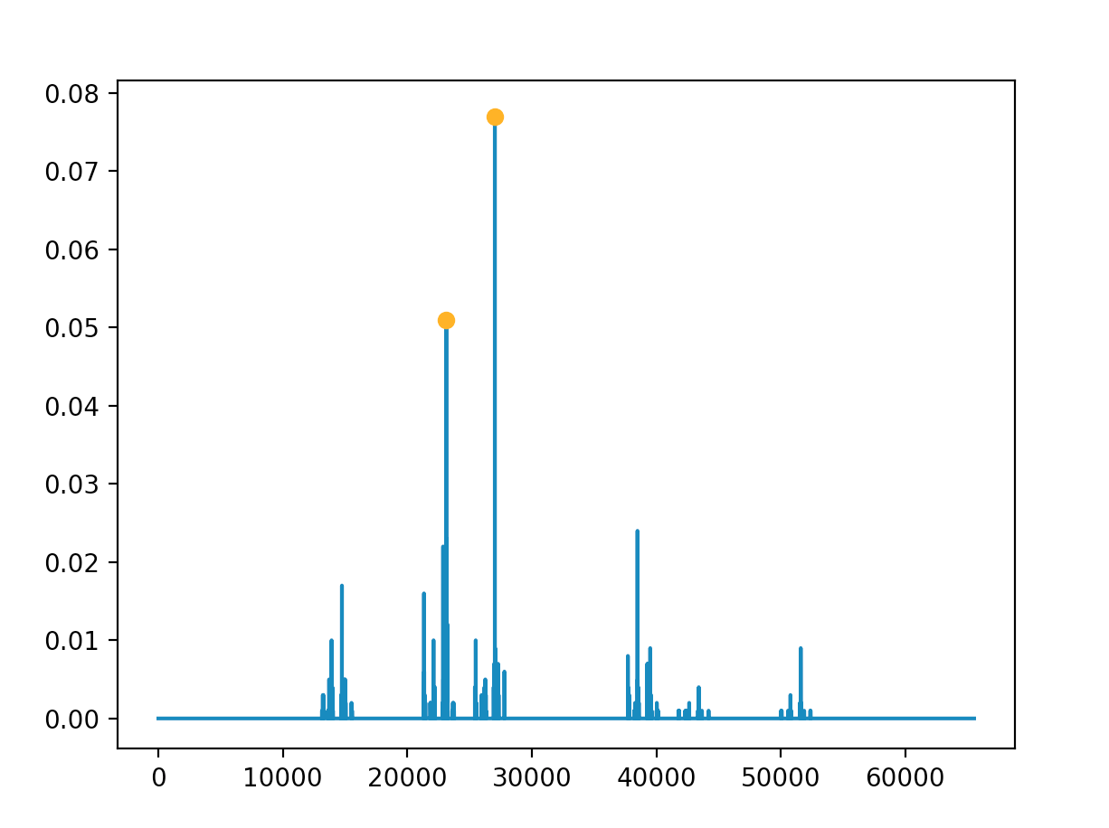
The tallest spikes (marked by the orange dots) in our simulation correspond to the states $|23130\rangle \ = \ |0101101001011010\rangle$ and $|27030\rangle \ = \ | 0110100110010110 \rangle$. The bitstrings map to the following adjacnecy matrices:

$$A_{23130} \ = \ \begin{pmatrix} 0 & 1 & 0 & 1 \\ 1 & 0 & 1 & 0 \\ 0 & 1 & 0 & 1 \\ 1 & 0 & 1 & 0 \end{pmatrix} \ \ \ \ \ \ \ \ \ A_{27030} \ = \ \begin{pmatrix} 0 & 1 & 1 & 0 \\ 1 & 0 & 0 & 1 \\ 1 & 0 & 0 & 1 \\ 0 & 1 & 1 & 0 \end{pmatrix}$$

The first adjacency matrix represents the outer ring around the graph (as you can check), which has cost $5 \ + \ 4 \ + \ 2 \ + \ 7 \ = \ 18$. The second adjacency matrix represents the "more horizontal" hourgalss cycle within the graph, which has cost $5 \ + \ 8 \ + \ 2 \ + \ 3 \ = \ 18$. We can quickly check the cost of the one remaining cycle within our graph, which is the "more horizontal" hourglass structure (its cost is $7 \ + \ 3 \ + \ 8 \ + \ 4 \ = \ 22$), verifying that our simulation has converged on the optimal solutions! It is important to note that like the first simulation, this simulation more volatile than one would hope (it doesn't always converge, and requires the constrained parameter search space), but like I mentioned previously, I believe this can be fixed by making the previously outlined modifcations to the algorithm.

Conclusion: Graphs Graphs Everywhere

I want to end off this blog post by re-iterating the power of graph theory. Graphs are very general and very useful mathematical structures. Essential any system that involves multiple "agents", each of which are interacting with one another in different ways, a graph provides a really good (yet, very simplified) mathematical picture of what exactly is going on. The graphs that we investigated in this post didn't necessarily represent any system that we see in the real world, however, they could. For instance, ProteinQure and Xanadu, two Toronto-based startups released a two papers a little while back, one of which is using QAOA to solve the protein folding problem (by modelling proteins as graphs), and another which attempts to predict molecular docking using an approach to solving graph problems called Gaussian Boson Sampling. This is different from QAOA, but at the root, they were essentially trying to find the maximum clique of a molecular, to precict binding sites, which they theoretically could have just used QAOA MaxClique to find!

In addition to this cool work, I was recently scrolling through Twitter (probably procrastinating, when I should have been working on this blog post), and I came across a guy named Kyle Vogt, who just recently finished running 7 marathons on 7 continents in 81 hours. I enjoy running, but such an expedition would surely result in my painful and hasty demise before I even finished the first half of the first marathon, so I was naturally very impressed by this superhuman endeavour. I became even more impressed/intrigued when I came across the code that he used to plan his trip. To choose his path around the world, Vogt used a variant of the Travelling Salesman Problem. Through encoding a bunch of constraints like location of airports, physical connection to the mainland, and war-torn countries where there was a non-zero probability of his plane being shot down, he performed TSP between a bunch of cities/Antarctic research bases, and found the optimal route. Theoretically, if Vogt had enough qubits (which he wouldn't, at least with current quantum computational devices), Vogt could have observed a computational speedup when planning his trip by using TSP! So as you can so, there are (theoretical, painfully theoretical) applications everywhere, ranging from modelling proteins, to planning an ultra-ultra-ultra marathon.

Hopefully this post was somewhat illuminating, and maybe even inspired you to come up with your own graph-theoretic combinatorial problems to crush with quantum algorithms!

---

Thanks for reading! For more content like this, check out the homepage of my website!